Example: Analysis of Emissions-Reduction Policy

U.S. Nationally Defined Contribution to Paris Accord

The United States’s Nationally Determined Contribution (NDC) to the 2015 Paris climate accord committed to reducing greenhouse gas emissions to 26–28% below 2005 levels by 2025 and with a longer-term target of reducing emissions to 80% below 2005 levels by 2050 (United States of America 2015).¹ This vignette will compare what these goals imply for rates of improving energy efficiency and transitioning from fossil fuels to clean energy sources. The methods will follow Roger Pielke, Jr.’s approach for both bottom-up and top-down analysis (Pielke 2009b, 2009a, 2010, 2011).

Bottom-Up Analysis

Pielke’s analysis rely on the Kaya identity: $F = P \times g \times e \times f,$ where

F is energy-related CO₂ emissions (here, measured in billions of metric tons),
P is the population in billions,
g is per-capita GDP (here, measured in thousands of dollars),
e is the energy intensity of the economy (here, measured in quads of primary energy consumed per trillion dollars of GDP²),
and f is the carbon intensity of the energy supply (here, measured in millions of metric tons of CO₂ per quad).

Pielke begins his bottom-up analysis by examining projections of future population and per-capita GDP. In this vignette, I develop those projections not from demographic and economic models, but simply by extrapolating from recent trends.

Recent Trends in Population and GDP

Begin by loading historical values of the Kaya identity parameters for the United States:

suppressPackageStartupMessages({
  library(magrittr)
  library(dplyr)
  library(stringr)
  library(tidyr)
  library(purrr)
  library(broom)
  library(knitr)
  library(scales)
  library(kayadata)
})

kaya <- get_kaya_data("United States")

Let’s start by looking at trends in P, g, e, and f starting in 1990. I plot these with a log-scale on the y-axis because a constant growth rate produces exponential growth, so it should look linear on a semi-log plot.

plot_kaya(kaya, "P", log_scale = TRUE, start_year = 1990, trend_line = TRUE, 
          points = FALSE) +
  theme_bw()
#> Warning: No shared levels found between `names(values)` of the manual scale and the
#> data's size values.
#> No shared levels found between `names(values)` of the manual scale and the
#> data's size values.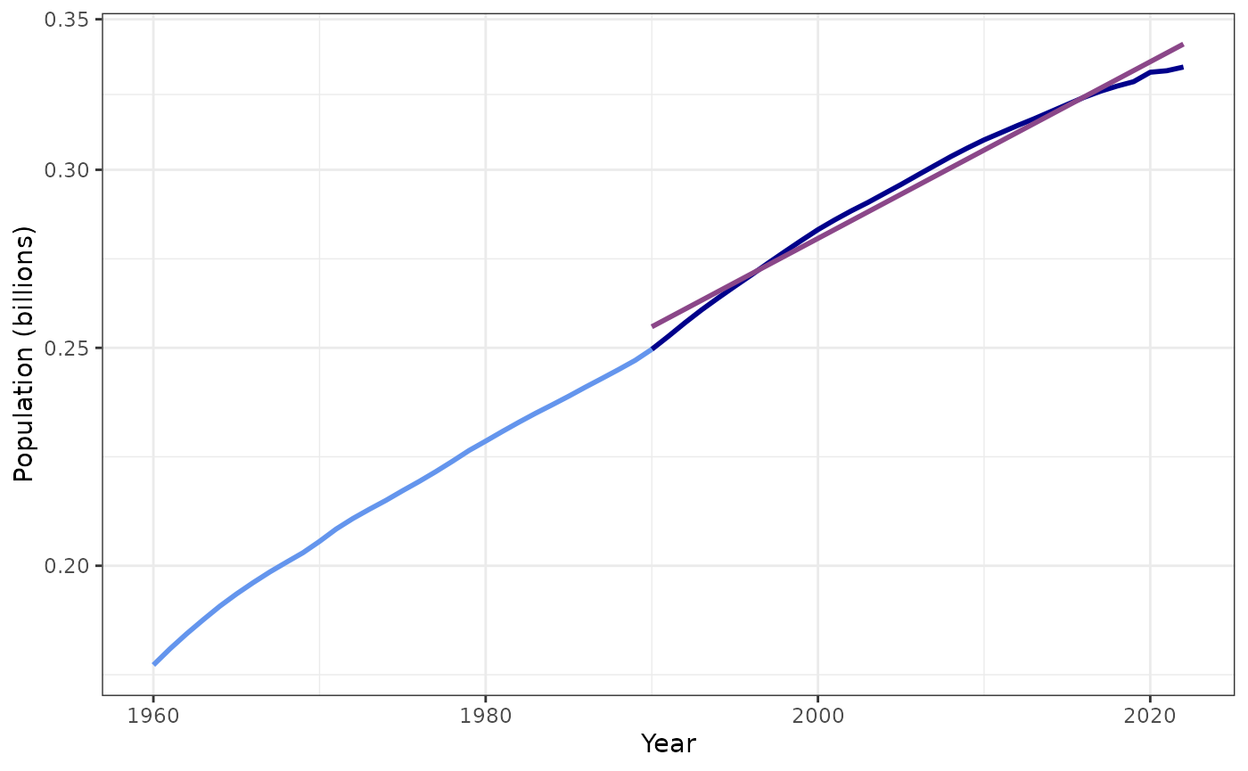

Trend in population for U.S. from 1990–2023

plot_kaya(kaya, "g", log_scale = TRUE, start_year = 1990, trend_line = TRUE, 
          points = FALSE) +
  theme_bw()
#> Warning: No shared levels found between `names(values)` of the manual scale and the
#> data's size values.
#> No shared levels found between `names(values)` of the manual scale and the
#> data's size values.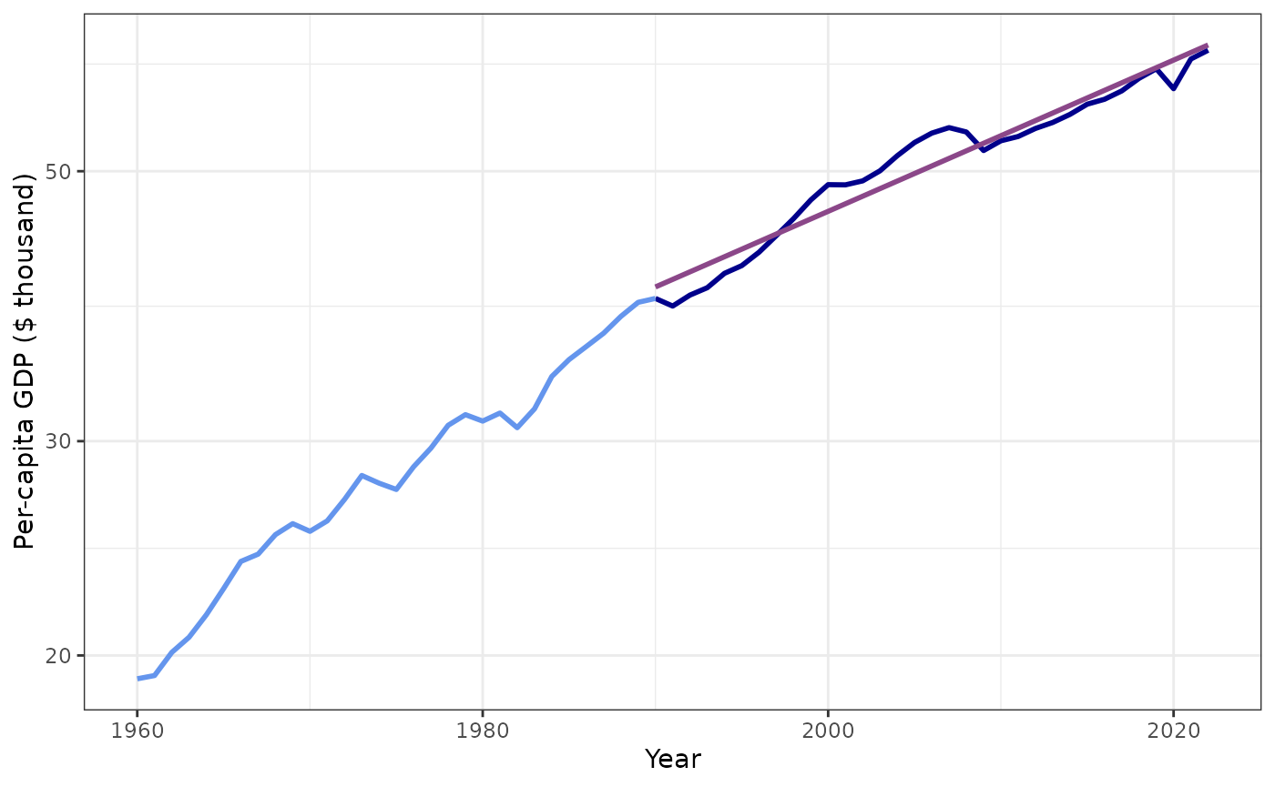

Trend in per-capita GDP for U.S. from 1990–2023

plot_kaya(kaya, "e", log_scale = TRUE, start_year = 1990, trend_line = TRUE, 
          points = FALSE) +
  theme_bw()
#> Warning: No shared levels found between `names(values)` of the manual scale and the
#> data's size values.
#> No shared levels found between `names(values)` of the manual scale and the
#> data's size values.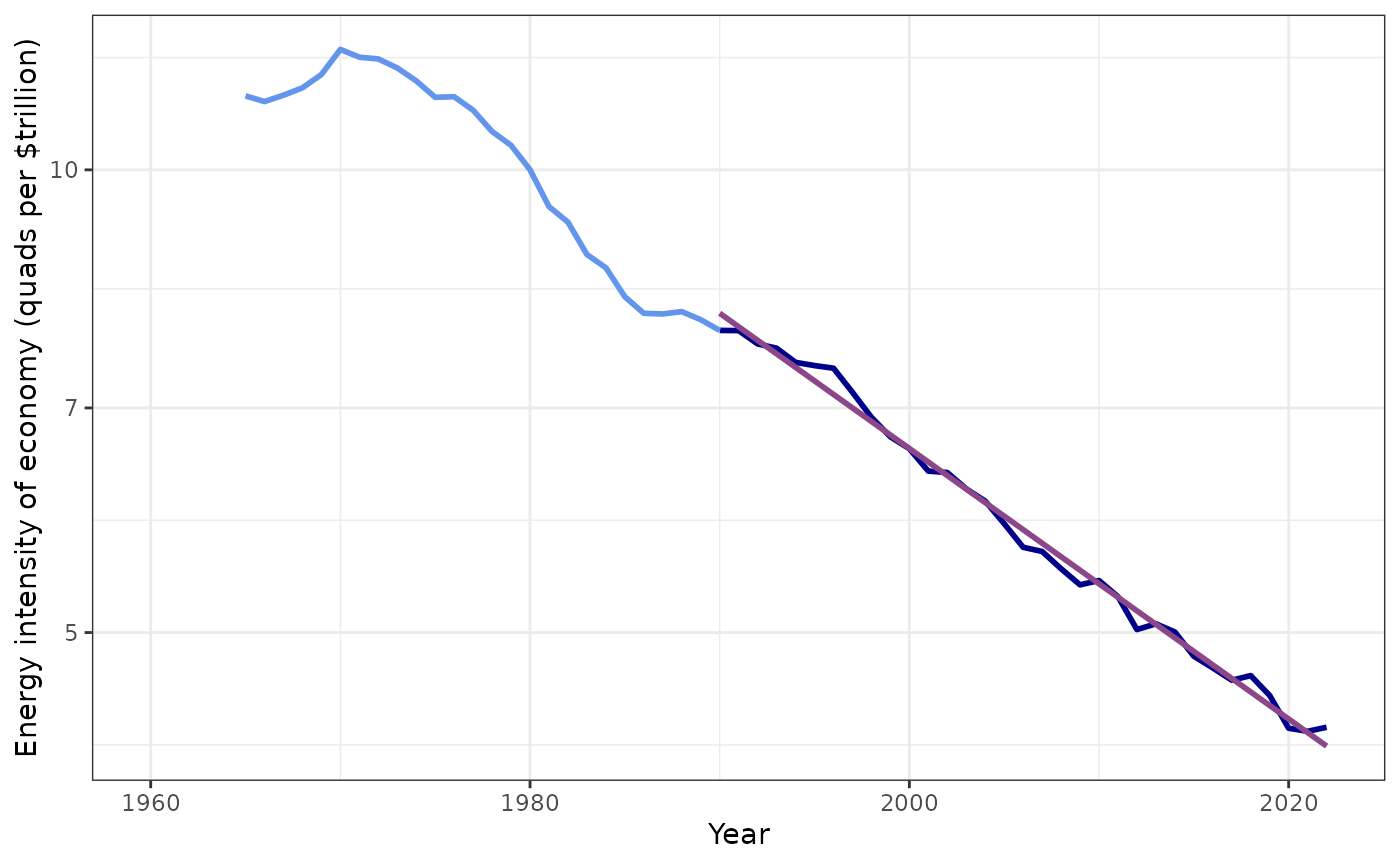

Trend in primary-energy intensity of the U.S. economy from 1990–2023

plot_kaya(kaya, "f", log_scale = TRUE, start_year = 1990, trend_line = TRUE, 
          points = FALSE) +
  theme_bw()
#> Warning: No shared levels found between `names(values)` of the manual scale and the
#> data's size values.
#> No shared levels found between `names(values)` of the manual scale and the
#> data's size values.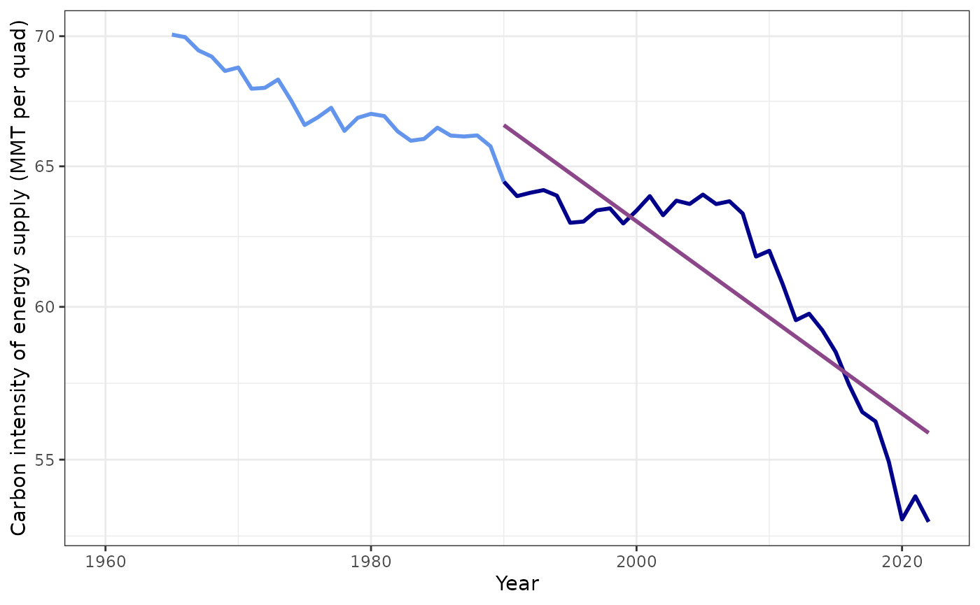

Trend in the carbon-dioxide intensity of the U.S. energy supply from 1990–2023

All of these trends look reasonable, except for f. Let’s try f again, but fitting the trend only since 2005:

plot_kaya(kaya, "f", log_scale = TRUE, start_year = 2005, trend_line = TRUE, 
          points = FALSE) +
  theme_bw()
#> Warning: No shared levels found between `names(values)` of the manual scale and the
#> data's size values.
#> No shared levels found between `names(values)` of the manual scale and the
#> data's size values.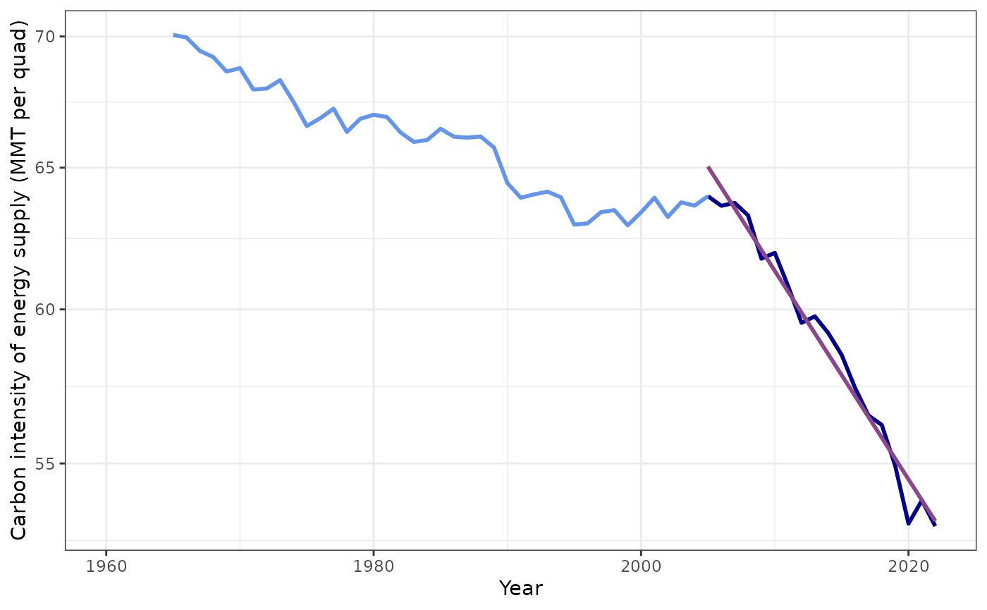

Trend in the carbon-dioxide intensity of the U.S. energy supply from 2005–2023

That looks better. The abrupt changes in trend at 1990 and again at 2005 illustrate the difficulties of predicting future values by extrapolating from past trends, and indicates that the extrapolations we will use here should be taken with several grains of salt.

Historical Trends

Now let’s calculate the historical trends:

vars <- c("P", "g", "e", "f")
historical_trends <- map_dbl(vars, 
                 ~kaya %>% 
                   gather(key = variable, value = value, -region, -year) %>%
                   filter(variable == .x, 
                          year >= ifelse(.x == "f", 2005, 1990)) %>%
                   lm(log(value) ~ year, data = .) %>% tidy() %>%
                   filter(term == "year") %$% estimate
) %>% set_names(vars)

tibble(Variable = names(historical_trends), 
       Rate = map_chr(historical_trends, ~percent(.x, 0.01))) %>%
  kable(align = c("c", "r"))

Variable	Rate
P	0.89%
g	1.48%
e	-2.08%
f	-1.20%

Implied Decarbonization Rates

Next, calculate the implied rate of change of F under the policy. This is not an extrapolation from history, but a pure implication of the policy goals: From the Kaya identity, $F = G \times e \times f$ , so the rates of change are $r_F = r_G + r_e + r_f = r_G + r_{ef}$ .

ref_year <- 2005
target_years <- c(2025, 2050)
target_reduction <- c(0.26, 0.80)

F_ref <- kaya %>% filter(year == ref_year) %$% F
F_target <- tibble(year = target_years, F = F_ref * (1 - target_reduction)) %>%
  mutate(implied_rate = log(F / F_ref) / (year - ref_year))

F_target %>% 
  mutate(implied_rate = map_chr(implied_rate, ~percent(.x,  0.01))) %>%
  rename("Target F" = F, "Implied Rate" = implied_rate) %>%
  kable(align = c("crr"), digits = 0)

year	Target F	Implied Rate
2025	4347	-1.51%
2050	1175	-3.58%

For the bottom-up analysis of decarbonization, I will use $r_{ef}$ , the implied rate of decarbonization of the economy, conditional on future economic growth following the historical trend. This is expressed in the equation $r_{ef} = r_F - r_G$ , where $r_F$ is the rate of emissions-reduction implied by the policy (see above) and $r_G$ is the historical growth rate of GDP:

implied_decarb_rates <- F_target %>% 
  transmute(year, impl_F = implied_rate, 
            hist_G = historical_trends['P'] + historical_trends['g'],
            hist_ef = historical_trends['e'] + historical_trends['f'],
            impl_ef = impl_F - hist_G)

implied_decarb_rates %>% 
  mutate_at(vars(starts_with("hist_"), starts_with("impl_")),
            list(~map_chr(., ~percent(.x, 0.01)))) %>%
  select(Year = year, 
         "implied F" = impl_F, 
         "historical G" = hist_G,
         "implied ef" = impl_ef, 
         "historical ef" = hist_ef
  ) %>%
  kable(align="rrrrr")

Year	implied F	historical G	implied ef	historical ef
2025	-1.51%	2.37%	-3.88%	-3.28%
2050	-3.58%	2.37%	-5.95%	-3.28%

Results

To meet the goals for 2025 would require increasing the rate of reducing ef from -3.28% per year to -3.88% per year: 1.2 times faster.

To meet the goals for 2050 would require increasing the rate of reducing ef from -3.28% per year to -5.95% per year: 1.8 times faster.

Top-Down Analysis

The top-down analysis is very similar to the bottom-up analysis, but instead of looking at the elements of the Kaya identity individually, we use predictions from macroeconomic integrated assessment models that consider interactions between population, GDP, and energy use to predict future energy demand:

top_down_trends <- get_top_down_trends("United States")

top_down_trends %>% select(P, G, E) %>%
  mutate_all(list(~map_chr(., ~percent(.x, 0.01)))) %>%
  rename("P trend" = P, "G trend" = G, "E trend" = E) %>%
  kable(align="rrr")

P trend	G trend	E trend
0.50%	1.90%	0.20%

Implied Decarbonization

In the bottom-up analysis, we calculated the implied rate of decarbonizing the economy by comparing the rate of emissions reduction implied by the policy ( $r_F$ ) to the predicted rate of change of GDP ( $r_G$ ). Here, in the top-down analysis, we calculate the implied rate of decarbonizing the energy supply ( $r_f$ ) by comparing the rate of emissions-reduction implied by policy ( $r_F$ ) to the predicted rate of growth of energy demand ( $r_E$ ): $F = E \times f$ , so $r_F = r_E + r_f$ , which we rearrange to find that $r_f = r_F - r_E$ .

implied_decarb_rates_top_down <- F_target %>% 
  transmute(year, impl_F = implied_rate, 
            top_down_E = top_down_trends$E,
            hist_f = historical_trends['f'],
            impl_f = impl_F - top_down_E)

implied_decarb_rates_top_down %>% 
  mutate_at(vars(starts_with("hist_"), starts_with("impl_"), 
                 starts_with("top_down")),
            list(~map_chr(., ~percent(.x, 0.01)))) %>%
  select(Year = year, 
         "implied F" = impl_F, 
         "top-down E" = top_down_E,
         "implied f" = impl_f, 
         "historical f" = hist_f
  ) %>%
  kable(align="rrrrr")

Year	implied F	top-down E	implied f	historical f
2025	-1.51%	0.20%	-1.71%	-1.20%
2050	-3.58%	0.20%	-3.78%	-1.20%

Results

To meet the goals for 2025 would require increasing the rate of reducing f from -1.20% per year to -1.71% per year: 1.4 times faster.

To meet the goals for 2050 would require increasing the rate of reducing f from -1.20% per year to -3.78% per year: 3.1 times faster.

References

Pielke, Roger A., Jr. 2009a. “Mamizu Climate Policy: An Evaluation of Japanese Carbon Emissions Reduction Targets.” Environmental Research Letters 4(4): 044001.

———. 2009b. “The British Climate Change Act: A Critical Evaluation and Proposed Alternative Approach.” Environmental Research Letters 4(2): 024010.

———. 2010. The Climate Fix: What Scientists and Politicians Won’t Tell You about Global Warming. Basic Books.

———. 2011. “An Evaluation of the Targets and Timetables of Proposed Australian Emissions Reduction Policies.” Environmental Science & Policy 14(1): 20–27.

United States of America. 2015. U.S. Cover Note, INDC, and Accompanying Information. https://www4.unfccc.int/sites/submissions/INDC/Published%20Documents/United%20States%20of%20America/1/U.S.%20Cover%20Note%20INDC%20and%20Accompanying%20Information.pdf.

The Trump administration has announced its intention to withdraw from the Paris accord. The analysis in this vignette does not address that development and simply presents the implications of the pledged contribution.↩︎
A quad is short for a quadrillion British Thermal Units.↩︎

Jonathan Gilligan

2019-07-31

U.S. Nationally Defined Contribution to Paris Accord

Bottom-Up Analysis

Recent Trends in Population and GDP

Historical Trends

Implied Decarbonization Rates

Results

Top-Down Analysis

Implied Decarbonization

Results

References