Introduction to datafsm

Abstract

The datafsm package implements a method for automatically generating models of dynamic processes that both have strong predictive power and are interpretable in human terms. We use an efficient model representation and a genetic algorithm-based estimation process. This paper offers a brief overview of the software and demonstrates how to use it.

Introduction

This package implements our method for automatically generating models of dynamic decision-making that both have strong predictive power and are interpretable in human terms. We use an efficient model representation and a genetic algorithm-based estimation process to generate simple deterministic approximations that explain most of the structure of complex stochastic processes. The genetic algorithm is implemented with the GA package (Scrucca 2013). Our method, implemented in C++ and R, scales well to large data sets. We have applied the package to empirical data, and demonstrated the method’s ability to recover known data-generating processes by simulating data with agent-based models and correctly deriving the underlying decision models for multiple agent models and degrees of stochasticity.

A user of our package can estimate models by providing their data in a common “panel data” format. The package is designed to estimate time series classification models that use a small number of binary predictor variables and move back and forth between the values of the outcome variable over time. Larger sets of predictor variables can be reduced to smaller sets with cross-validation. Although the predictor variables must be binary, a quantitative variable can be converted into binary by division of the observed values into high/low classes. Future releases of the package may include additional estimation methods to complement genetic algorithm optimization.

# Load and attach datafsm into your R session, making its functions available:
library(datafsm)

Please cite the package if you use it with the text generated by:

citation("datafsm")

## To cite package 'datafsm' in publications use:
## 
##   Nay JJ, Gilligan JM (2015). "Data-driven dynamic decision models." In
##   Yilmaz L, Chan WKV, Moon I, Roeder TMK, Macal C, Rosetti M (eds.),
##   _Proceedings of the 2015 Winter Simulation Conference_, 2752-2763.
##   doi:10.1109/WSC.2015.7408381
##   <https://doi.org/10.1109/WSC.2015.7408381>.
## 
## A BibTeX entry for LaTeX users is
## 
##   @InProceedings{,
##     title = {Data-driven dynamic decision models},
##     author = {John J. Nay and Jonathan M. Gilligan},
##     booktitle = {Proceedings of the 2015 Winter Simulation Conference},
##     year = {2015},
##     editor = {L. Yilmaz and W. K. V. Chan and I. Moon and T. M. K. Roeder and C. Macal and M. Rosetti},
##     pages = {2752--2763},
##     doi = {10.1109/WSC.2015.7408381},
##   }

Fake Data Example

To quickly show it works, we can create fake data. Here, we generate 1000 repetitions of a 10-round game in which each player starts by making a random move, and in subsequent rounds, each player follows a “noisy tit-for-tat” strategy that’s equivalent to tit-for-tat, except that with a 5% probability the player will make a random move.

rounds <- 10
reps <- 1000
noise_level <- 0.05

seed1 <- 1372456261
seed2 <-  597693057
seed3 <-  805078823
set.seed(seed1)
cdata <- data.frame(outcome = NA,
                    period = rep(seq(rounds), reps),
                    my.decision1 = NA,
                    other.decision1 = NA)

#
# Prisoner's dilemma
#
pd_outcome <- function(player_1, player_2) {
  #
  # 1 = C
  # 2 = D
  #
  player_1  + 1
}

tit_for_tat <- function(last_round_self, last_round_opponent) {
    last_round_opponent
}

noisy_tit_for_tat <- function(last_round_self, last_round_opponent, noise_level) {
  if (runif(1,0,1) <= noise_level) {
    sample(0:1,1)
  } else {
    last_round_opponent
  }
}

for (i in seq_along(cdata$period)) {
  if (cdata$period[i] == 1) {
    my.decision <- sample(0:1,1, prob = c(1 - noise_level, noise_level))
    other.decision <- sample(0:1,1, prob = c(1 - noise_level, noise_level))
    cdata[i, "outcome"] <- pd_outcome(my.decision, other.decision)
  } else{
    my.last <- my.decision
    other.last <- other.decision
    my.decision <- noisy_tit_for_tat(my.last, other.last, noise_level)
    other.decision <- noisy_tit_for_tat(other.last, my.last, noise_level)
    cdata[i,c("outcome", "my.decision1", "other.decision1")] <- 
      c(pd_outcome(my.decision, other.decision), my.last, other.last)
  }
}

The only required argument of the main function of the package, evolve_model, is a data.frame object, which must have 3-5 columns. The first two columns must be named period and outcome (period is the time period that the outcome action was taken). The remaining one to three columns are predictors, and may have arbitrary names. Each row of the data.frame is an observational unit, an action taken at a particular time and any relevant variables for that time. All of the (3-5 columns) should be named. The period and outcome columns should be integer vectors — e.g. c(1,2,1) — and the columns with the predictor variable data should be logical vectors — e.g. c(TRUE, FALSE, FALSE) — or vectors that can be coerced to logical with as.logical().

Here are the first eleven rows of this fake data:

outcome	period	my.decision1	other.decision1
1	1	NA	NA
1	2	0	0
1	3	0	0
2	4	0	0
1	5	1	0
2	6	0	1
1	7	1	0
2	8	0	1
1	9	1	0
2	10	0	1
1	1	NA	NA

We can estimate a model with that data. evolve_model uses a genetic algorithm to estimate a finite-state machine (FSM) model, primarily for understanding and predicting decision-making. This is the main function of the datafsm package. It relies on the GA package for genetic algorithm optimization. We chose to use a GA because GAs perform well in rugged search spaces to solve integer optimization problems, are a natural complement to our binary representation of FSMs, and are easily parallelized.

evolve_model takes data on predictors and data on the outcome and automatically creates a fitness function that takes training data, an action vector that evolve_model generates, and a state matrix evolve_model generates as input and returns numeric vector whose length is the number of rows in the training data. evolve_model then computes a fitness score for that potential solution FSM by comparing it to the provided outcome in the real training data. This is repeated for every FSM in the population and then the probability of selection for the next generation is proportional to the fitness scores. If the argument cv is set to TRUE the function will call itself recursively while varying the number of states inside a cross-validation loop in order to estimate the optimal number of states, then it will set the number of states to that optimal number and estimate the model on the full training set.

If the argument parallel is set to TRUE, then these evaluations are distributed across the available processors of the computer using the doParallel functions; otherwise, the evaluations of fitness are conducted sequentially. Because this fitness function that evolve_model creates must loop through all the training data every time it is evaluated and we need to evaluate many possible solution FSMs, the fitness function is implemented in C++ to improve its performance.

set.seed(seed2)
res <- evolve_model(cdata, seed = seed3)

evolve_model evolves the models on training data and then, if a test set is provided, uses the best solution to make predictions on test data. Finally, the function returns the GA object and the decoded version of the best string in the population. Formally, the function return an S4 object with slots for:

call Language from the call of the function.
actions Numeric vector with the number of actions.
states Numeric vector with the number of states.
GA S4 object created by ga() from the GA package.
state_mat Numeric matrix with rows as states and columns as predictors.
action_vec Numeric vector indicating what action to take for each state.
predictive Numeric vector of length one with test data accuracy if test data was supplied; otherwise, a character vector with a message that the user should provide test data for better estimate of generalizable performance.
varImp Numeric vector with length equal to the number of columns in the state matrix, containing relative importance scores for each predictor.
timing Numeric vector length one containing the total elapsed time it took evolve_model to execute.
diagnostics Character vector length one, designed to be printed with base::cat().

Use the summary and plot methods on the output of the evolve_model() function:

summary(res)

## Length  Class   Mode 
##      1 ga_fsm     S4

plot(res, action_label = ifelse(action_vec(res)==1, "C", "D"), 
     transition_label = c('cc','dc','cd','dd'))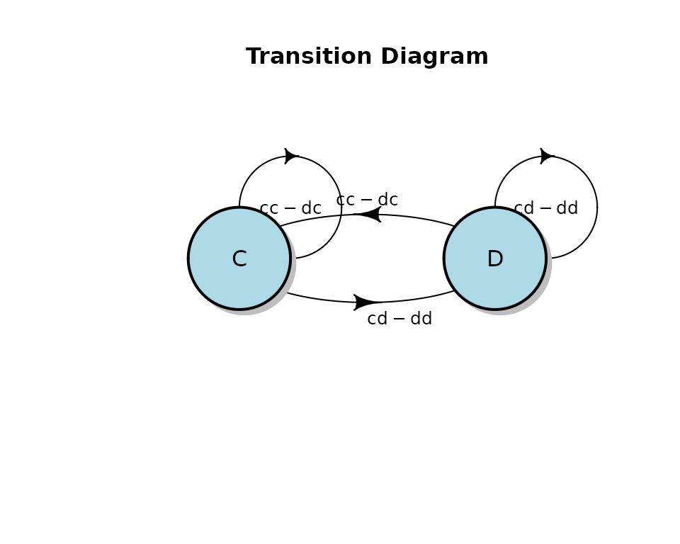

Result of plot() method call on ga_fsm object.

The diagram shows that evolve_model recovered a tit-for-tat model in which the player in question (“me”) mimics the last action of the opponent.

Use the estimation_details method on the output of the evolve_model() function:

suppressMessages(library(GA))
plot(estimation_details(res))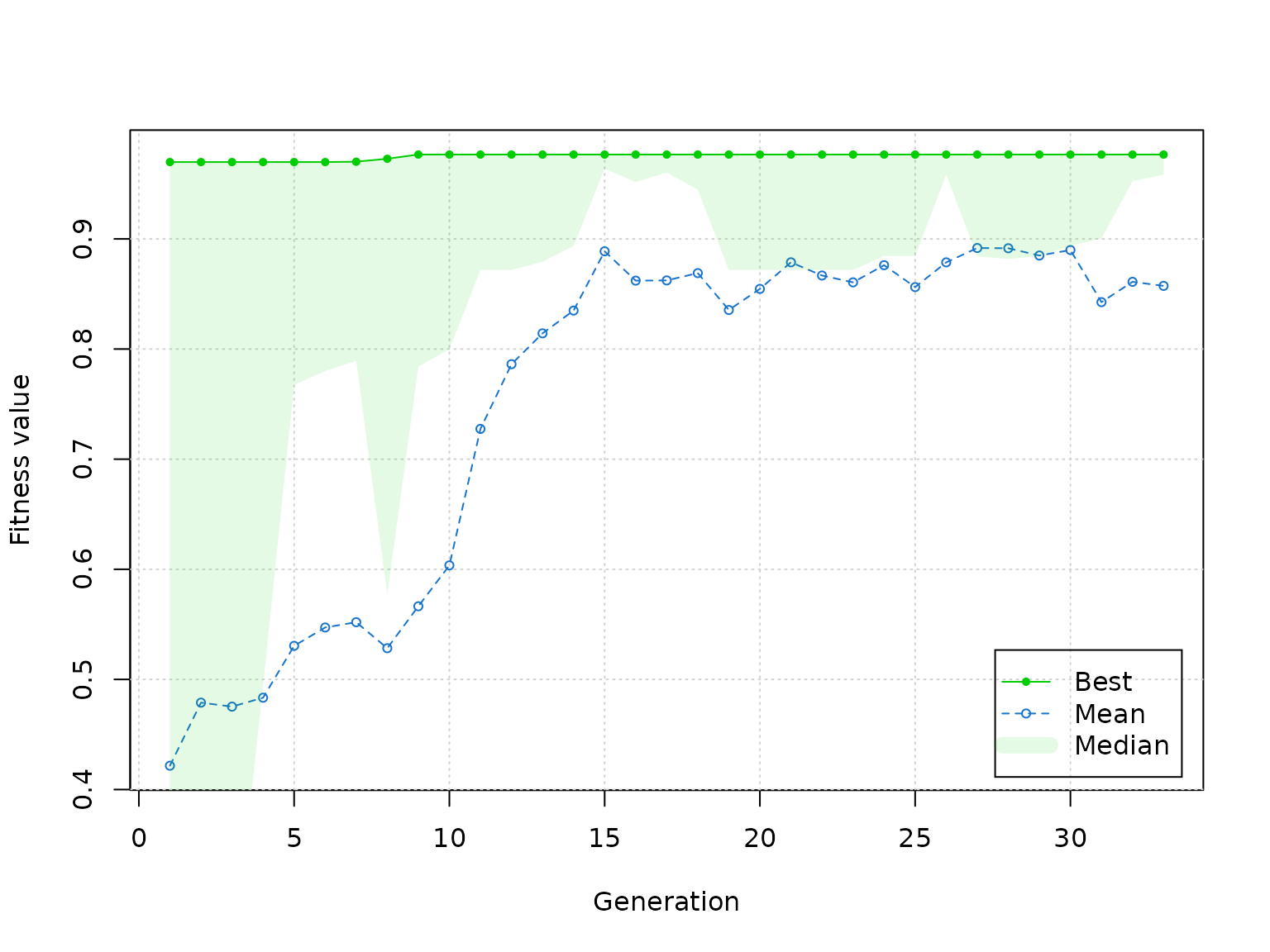

Result of plot() method call on ga object, which is obtained by calling estimation_details() on ga_fsm object.

Documentation for `evolve_model`

Check out the documentation for the main function of the package to learn about all the options:

?evolve_model

Acknowledgments

This work is supported by U.S. National Science Foundation grants EAR-1416964 and EAR-1204685.

Session Info

sessionInfo()

## R version 4.5.2 (2025-10-31)
## Platform: x86_64-pc-linux-gnu
## Running under: Ubuntu 24.04.3 LTS
## 
## Matrix products: default
## BLAS:   /usr/lib/x86_64-linux-gnu/openblas-pthread/libblas.so.3 
## LAPACK: /usr/lib/x86_64-linux-gnu/openblas-pthread/libopenblasp-r0.3.26.so;  LAPACK version 3.12.0
## 
## locale:
##  [1] LC_CTYPE=C.UTF-8       LC_NUMERIC=C           LC_TIME=C.UTF-8       
##  [4] LC_COLLATE=C.UTF-8     LC_MONETARY=C.UTF-8    LC_MESSAGES=C.UTF-8   
##  [7] LC_PAPER=C.UTF-8       LC_NAME=C              LC_ADDRESS=C          
## [10] LC_TELEPHONE=C         LC_MEASUREMENT=C.UTF-8 LC_IDENTIFICATION=C   
## 
## time zone: UTC
## tzcode source: system (glibc)
## 
## attached base packages:
## [1] stats     graphics  grDevices utils     datasets  methods   base     
## 
## other attached packages:
## [1] GA_3.2.4         iterators_1.0.14 foreach_1.5.2    datafsm_0.2.5   
## 
## loaded via a namespace (and not attached):
##  [1] shape_1.4.6.1        gtable_0.3.6         xfun_0.54           
##  [4] bslib_0.9.0          ggplot2_4.0.1        recipes_1.3.1       
##  [7] lattice_0.22-7       vctrs_0.6.5          tools_4.5.2         
## [10] generics_0.1.4       stats4_4.5.2         parallel_4.5.2      
## [13] tibble_3.3.0         ModelMetrics_1.2.2.2 pkgconfig_2.0.3     
## [16] Matrix_1.7-4         data.table_1.17.8    RColorBrewer_1.1-3  
## [19] S7_0.2.1             desc_1.4.3           lifecycle_1.0.4     
## [22] stringr_1.6.0        compiler_4.5.2       farver_2.1.2        
## [25] textshaping_1.0.4    diagram_1.6.5        codetools_0.2-20    
## [28] htmltools_0.5.8.1    class_7.3-23         sass_0.4.10         
## [31] yaml_2.3.10          prodlim_2025.04.28   pillar_1.11.1       
## [34] pkgdown_2.2.0        crayon_1.5.3         jquerylib_0.1.4     
## [37] MASS_7.3-65          cachem_1.1.0         gower_1.0.2         
## [40] rpart_4.1.24         nlme_3.1-168         parallelly_1.45.1   
## [43] lava_1.8.2           tidyselect_1.2.1     digest_0.6.39       
## [46] stringi_1.8.7        future_1.68.0        reshape2_1.4.5      
## [49] dplyr_1.1.4          purrr_1.2.0          listenv_0.10.0      
## [52] splines_4.5.2        fastmap_1.2.0        grid_4.5.2          
## [55] cli_3.6.5            magrittr_2.0.4       survival_3.8-3      
## [58] future.apply_1.20.0  withr_3.0.2          scales_1.4.0        
## [61] lubridate_1.9.4      timechange_0.3.0     rmarkdown_2.30      
## [64] globals_0.18.0       nnet_7.3-20          timeDate_4051.111   
## [67] ragg_1.5.0           evaluate_1.0.5       knitr_1.50          
## [70] hardhat_1.4.2        caret_7.0-1          doParallel_1.0.17   
## [73] rlang_1.1.6          Rcpp_1.1.0           glue_1.8.0          
## [76] pROC_1.19.0.1        ipred_0.9-15         jsonlite_2.0.0      
## [79] R6_2.6.1             plyr_1.8.9           systemfonts_1.3.1   
## [82] fs_1.6.6

John J. Nay and Jonathan M. Gilligan