This document applies the datafsm software package (Nay and Gilligan 2015) to the data from Fudenberg, Rand, and Dreber (2012). For the motivation, underlying design, and tests on simulated data see Nay and Gilligan (2015). For a simple example of how to use the package see the “Introduction to datafsm” vignette.

library(dplyr)
library(tidyr)
library(purrr)
library(pander)
library(datafsm)
set.seed(1533406114)

Estimating a model is as simple as ensuring the input data, e.g. prepped, is in the correct format and calling evolve_model(prepped). Here, we loop through the six experimental treatments in the data and estimate a separate model for each, storing the results in a list we name res. The parallel argument allows this work to automatically be spread across all available processors on the computer. This parallelization, combined with the implementation of the core computation in C++, speeds up estimation considerably.

The datafsm package includes a dataset from Nay and Vorobeychik (2016), which represents 168,386 rounds of play in 30 different variations on the iterated prisoner’s dilemma game. This example will focus on the six games studied by Fudenberg, Rand, and Dreber (2012).

data(NV_games, package = "datafsm")

group_df <- list(g1 = 15, g2 = 16, g3 = 17, g4 = 14, g5 = 13, g6 = 12) %>%
  as_tibble() %>% pivot_longer(cols = everything(), names_to = "label",
                               values_to = "group") %>%
  mutate(group = as.integer(group))

prepped <- NV_games %>% transmute(
  group = as.integer(group),
  outcome = as.integer(my.decision == "coop") + 1,
  period = as.integer(period),
  my.decision1 = as.integer(my.decision1 == 1),
  other.decision1 = as.integer(other.decision1 == 1)
) %>%
  filter(group %in% group_df$group) %>%
  full_join(group_df, by = "group") %>%
  arrange(label) %>%
  select(-group) %>% rename(group = label)

group_indices <- prepped$group %>% unique() %>% sort()
group_seeds <- sample.int(.Machine$integer.max, length(group_indices)) %>%
  set_names(as.character(group_indices))

patterns <- NV_games %>% select(group, error, r, t) %>%
  mutate(group = as.integer(group)) %>%
  full_join(group_df, by = "group") %>%
  select(-group) %>% rename(group = label) %>%
  filter(group %in% group_indices) %>%
  group_by(group) %>% distinct() %>% ungroup() %>%
  arrange(group)

res <- lapply(as.list(group_indices), function(x){
  message("\nAnalyzing group ", x, "\n")
  prepped %>% filter(group == x) %>% select(-group) %>%
    evolve_model(parallel = TRUE,
                 seed = group_seeds[[as.character(x)]],
                 verbose = FALSE)
})

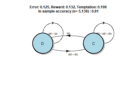
The resulting object has methods for inspecting (print, show, summary, estimation_details, best_performance, varImp, states), visualizing (plot, barplot, dotchart), and predicting new data (predict). Below we use the plot and barplot methods to see the resulting model and the associated relative importance of the predictor variables. In this case, the predictor variables are the outcomes of the decisions in the previous period of the game and the outcome variable (the current state) is the action the model predicts the agent will take in the current period. The state on the far left is the starting state.

The variable importance is computed by switching each value of an estimated model’s state matrix to another value in its feasible range, measuring the decrease in goodness of fit to the data, normalizing the values so the largest is 100, then summing across each column to estimate the relative importance of each predictor variable across all states.

names(res) <- group_indices
tl = c("dd", "cd", "dc", "cc")
for(name in names(res)){
  pattern <- patterns %>% filter(group == name)
  this_res <- res[[name]]
  plot(this_res,
       action_label = ifelse(action_vec(this_res)==1, "C", "D"),
       transition_label = tl,
       maintitle = paste0("Error: ", pattern$error,
                          ", Reward: ", pattern$r,
                          ", Temptation: ", pattern$t,
                          "\n In-sample accuracy (n= ",
                          formatC(sum(prepped$group==name),
                                  big.mark=',',digits=0),") : ",
                          round(best_performance(this_res),2)))

   barplot(this_res, names.arg=tl)
}

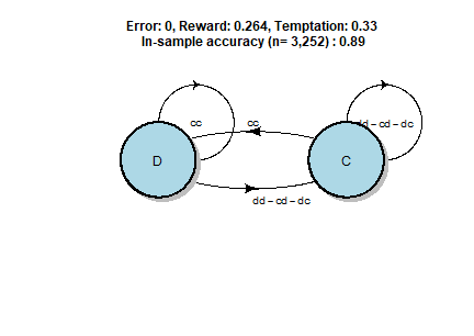
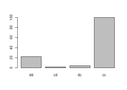
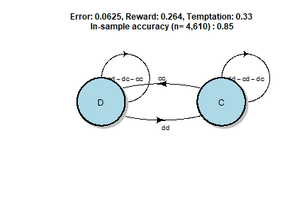
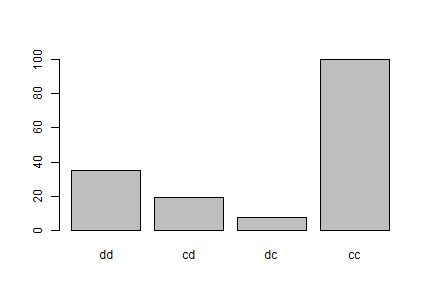
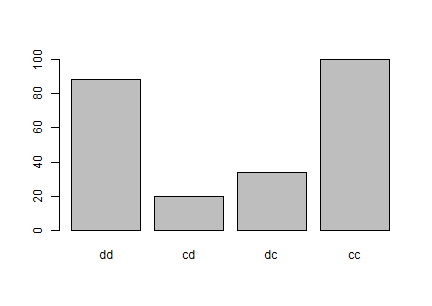
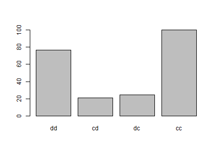
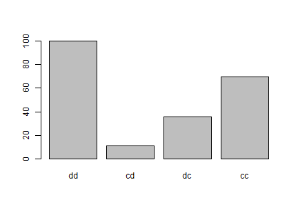
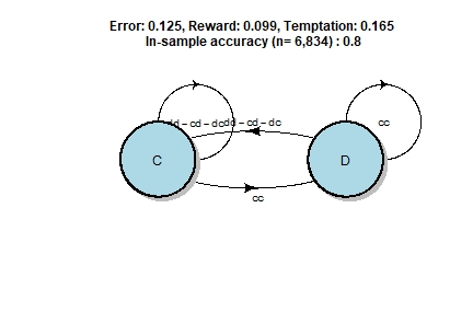
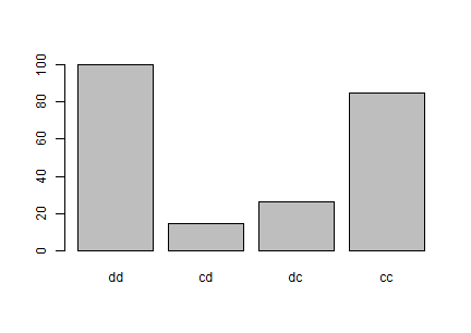plot of chunk plot_results These variable importance plots of the six models capture ways in which the game design affects player behavior. The first two models are from the games where the error is zero or low: the cc outcome is by far the strongest predictor of play. Compare this to the next four models where error is higher: the dd becomes much more important. Now compare the third and fourth models from games with payoffs more amenable to cooperation to the fifth and sixth models from games with payoffs less amenable to cooperation: the dd outcome is more important in the latter. We can summarize this main pattern with a table.

c_minus_d <- res %>% map_dbl(~varImp(.x)[4] - varImp(.x)[1])
df <- c_minus_d %>% as.list() %>% as_tibble() %>%
  pivot_longer(cols = everything(), names_to = "group",
               values_to = "c_minus_d") %>%
  full_join(patterns, by = "group") %>%
  select(error, r, t, c_minus_d) %>%
  rename(Error = error, Reward = r, Temptation = t,
         "CC Imp. Re. to DD" = c_minus_d)
pander(df)

Error	Reward	Temptation	CC Imp. Re. to DD
0	0.264	0.33	77.55
0.0625	0.264	0.33	65.16
0.125	0.264	0.33	12.09
0.125	0.165	0.231	23.68
0.125	0.132	0.198	-30.7
0.125	0.099	0.165	-15.37

These were all two-state models, which is the default. When we call evolve_model we can either manually set the number of states, states, or we can set the argument cv to TRUE, which then estimates the out-of-sample performance through k-fold cross-validation on the training data for many values of the number of states to determine the number of states with best out-of-sample performance for the given dataset (and the given split into k-folds, which it should be relatively insensitive to).

k_fold_seeds <- sample.int(.Machine$integer.max, length(group_indices)) %>%
  set_names(as.character(group_indices))
res2 <- lapply(as.list(group_indices), function(x){
  message("\nPerforming k-fold cross-validation for group ", x, "\n")
  # Note: When parallel is set TRUE, evolve_model processes the first few
  # groups successfully, but then GA::ga crashes with "mcfork() unable to
  # create pipe" when evolving the model for the third or fourth group
  # (the exact time it crashes varies from run to run on the same machine).
  # There is no similar problem when evolving models with parallel = TRUE
  # in the analyze_data chunk.
  cv_res <- prepped %>% filter(group == x) %>% select(-group) %>%
    evolve_model(parallel = FALSE,
                 cv = TRUE, max_states = 6, k = 5,
                 seed = k_fold_seeds[[as.character(x)]],
                 verbose = FALSE)
  message("\nFinished k-fold cross-validation for group ", x, "\n")
  cv_res
})

names(res2) <- group_indices
res2states <- map_dbl(res2, states) %>% as.integer() %>%
  set_names(names(res2)) %>% as.list() %>% as_tibble() %>%
  pivot_longer(cols = everything(), names_to = "group", values_to = "states")
df2 <- patterns %>% full_join(res2states, by = "group") %>%
  arrange(group) %>%
  select(Error = error, Reward = r, Temptation = t, States = states)
pander(df2)

Error	Reward	Temptation	States
0	0.264	0.33	2
0.0625	0.264	0.33	4
0.125	0.264	0.33	4
0.125	0.165	0.231	4
0.125	0.132	0.198	2
0.125	0.099	0.165	2

References

Fudenberg, Drew, David G Rand, and Anna Dreber. 2012. “Slow to Anger and Fast to Forgive: Cooperation in an Uncertain World.” American Economic Review 102 (2): 720–49. https://doi.org/10.1257/aer.102.2.720.

Nay, John J., and Jonathan M. Gilligan. 2015. “Data-Driven Dynamic Decision Models.” In Proceedings of the 2015 Winter Simulation Conference, 2752–63. IEEE Press. https://doi.org/10.1109/WSC.2015.7408381.

Nay, John J., and Yevgeniy Vorobeychik. 2016. “Predicting Human Cooperation.” PLOS ONE 11 (5): e0155656. https://doi.org/10.1371/journal.pone.0155656.

Example with real data

John Nay

2015-08-20

References